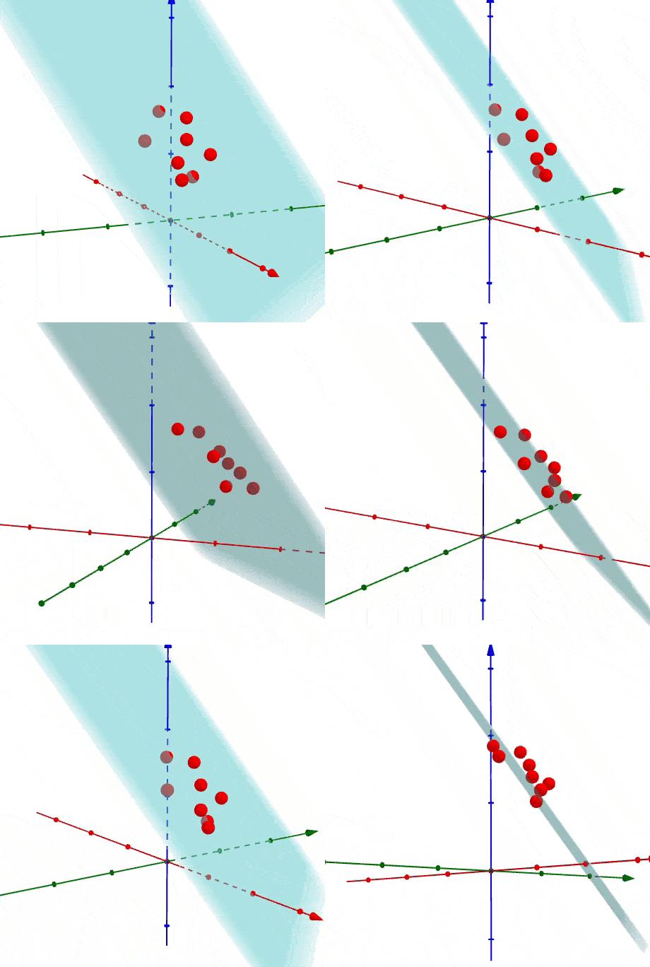
Imagine a world where there are more than 8 dimensions. Can you visualize it?
No?
That’s not surprising as we live in a world of three dimensions. However, in machine learning, you can have data across many variables, or dimensions, this is where dimensionality reduction comes into play.
Imagine now that you are trying to create a model with multiple variables. Much of the data you are looking to absorb into your model may not be relevant.
What is dimensionality reduction?
Dimensionality reduction is a process to remove certain variables from a data set that don’t add value to the output.
Removing dimensions with limited value is essential for running algorithms efficiently. The process allows you to get more from your analysis and scale.
There are two ways you can start using dimensionality reduction.
- Feature selection: This is the process where you select which variables to include in your algorithm manually. You can discount those you know to be irrelevant to the outcome you are trying to achieve.
- Feature projection: This second process is more mathematical. Here you are removing variables using algorithmic methods. There are multiple options for doing this, some of which are described below.
Why you need dimensionality reduction?
Before we get into the good stuff and different techniques of dimensionality reduction, it is necessary, we understand why we do it.
Machine learning can be an incredibly powerful way of gaining insights from data. However, the technology is not without its limitations.
There are three reasons why you would want to use dimensionality reduction for machine learning.
- Remove irrelevant information: You do not want to train an algorithm on data that is not relevant to the problem you are trying to solve. This could lead to poor insights and bad decisions.
- Simpler to complete analysis: When you have fewer variables, it makes it easier for the algorithm to converge. This allows you to get insights more quickly. This is great if you are trying to make business decisions that run on tight deadlines.
- Improve the efficiency of analysis: Machine learning is a very processor heavy tool. It needs a lot of power to complete. That is why it is crucial that you run the most efficient algorithm.
Different techniques
Ok, so we know what dimensionality reduction is and why it is useful. It’s now time to get into how to implement it for your data set.
PCA (Principal Component Analysis)
PCA is a statistical process via which you transform the matrix coordinates of your data points onto a linear plane.
Did you get that?
Yer, I realize that the sentence could be a little confusing!
Basically, all you need to know is that mathematical wizardry is performed that moves your data points so that you can linearly model them on a single axis. This process of dimensionality reduction makes it easier to run your analysis in production.
Do you remember learning about linear regression and how it was the simplest type of machine learning? Being able to analyze data in a linear system makes it simpler to process.
This article explains the wizardry in an easy to digest way if you want to learn more.

FYI This is probably the most common way people implement dimensionality reduction. So if you’re happy with this, then you can probably stop reading for the time being.
You can implement PCA in python using the following code.
Skip to the next section though to understand where dimensionality reduction can be harmful.
NMF (non-negative matrix factorization)
Non-negative matrix factorization is another technique with a super fun name.
Non-negative just sounds wrong, am I right?
In this technique, your matrix of data points is converted into multiple, usually two vectors, W and H.
In splitting out the matrix into the two vectors, all negative data points are removed. This makes the process of completing analysis on the data simpler.
You can read more about the process of NMF here.
Kernels for Data Transform
I have covered kernels in a previous post.
As with PCA described above, some mathematical wizardry is performed on the data set that allows you to project the information in a linear plane.
One example is the Gaussian kernel.
This performs a Gaussian function on the data, converting it to a new dimension that is linearly separable. Then when you project the data back onto a lower dimension, you can analyze it linearly.
You can in fact use kernels within PCA analysis directly. The process is called Kernel PCA (shocking I know).
Below you can see how to implement kernel PCA using the Scikit Learn library. You apply the Kernel PCA to the training data set and then train your ML algorithm as usual.
Don’t worry if you don’t fully understand what I just said, you can read more details here.
K-Nearest neighbours
Another way of simplifying analysis is by only looking at the data points closest to the prediction you are trying to make.
One example of this in action is K-Nearest Neighbours analysis.
By looking at a reduced data set for your prediction you are removing dimensions, and simplifying the process.
I covered K-Nearest Neighbours in this article if you want more information on it.
Decision Trees and Random Forest Analysis
Other algorithms take out dimensions from your data automatically when making predictions.
As with the other techniques we have covered today for dimensionality reduction, this process uses some pretty sophisticated mathematics.
If you are interested to understand more about how this works, you can get an overview of both decision tree and random forest analysis in this post.
Backward Feature Elimination
The final technique on dimensionality reduction we will cover today is backward feature elimination.
This process involves running your algorithm on a training set and then systematically going back to remove one variable at a time and see the impact.
It is a fairly involved process, but in the end, you should only have variables in the algorithm that are significant.
This is important when you start to use the algorithm on new data as it will be more efficient.
Learn more about backward elimination here.
When can dimensionality reduction be bad?
So far we have sung the praised of dimensionality reduction as the solution to all your algorithm woes. But it’s not all blue skies and sunshine. Sometimes dimensionality reduction can be harmful.
Here are three examples of where dimensionality reduction is terrible:
- Loss of data: You have worked so hard to get a thorough data set. It’s a shame to be losing some of this valuable data; furthermore, it can mean that you miss something meaningful for your analysis.
- Algorithms not always right: As with all predictive and algorithmic techniques, the algorithms used in dimensionality reduction are not consistently right. Sometimes these processes will cause you to focus on the wrong inputs.
- Reduce accuracy: It is likely that implementing PCA or one of the other techniques described above will reduce your accuracy. This is something you need to balance against the efficiency gains we described previously.
So that about covers dimensionality reduction.
This is an important technique that will allow you to run better projects with machine learning.
Ready to get started with Machine Learning Algorithms? Try the FREE Bootcamp
To Summarise on Dimensionality Reduction
The clue is in the name, dimensionality reduction reduces the number of dimensions (or variables) in your data set. This simplifies your analysis.
The main technique people use PCA (Principal Component Analysis) which can be implemented directly using libraries available in python such as Scikit Learn.
Despite the benefits, it is also vital you understand the risks. When you can critically analyze how dimensionality reduction is working for your project, you will win.
Powerful and efficient machine learning algorithms are available to you.
What will you discover?
Advertising Disclosure: I an affiliate of Udemy and may be compensated in exchange for clicking on the links posted on this website. I only advertise for course I have found valuable and think will help you too.
If you have found this content helpful, I recommend the course linked below which gave me a baseline understanding of the materials and python code shared here.
Machine Learning A-Z: Hands-On Python & R In Data Science


